As modern day product become increasingly complex one must be conscious of all the featural characteristics that define its employment and value; these are basically raised by the potential market. The producer is compelled to translate these consumer concerns into technical requirements; which are always bound to quantification. These elements will be seen as manageable outputs derived from the activities that hold up the organization. One must strive to visualize these, as prime materials for the drafting mission statements within companies.

The upcoming piece will demonstrate that through the thorough appliance of statistical tools and Quality Function Design (DFMEA) thinking, one can depart from public data to distil value according to market demands; by compounding it with six sigma, one can backwardly flesh out the product endgame from the clients necessities to its conceptual inception, and its subsequent operation, as this work will explain. The paramount tenet of quality control and the Quality Function Design (QFD) is to understand that these market demands stem out from manageable variables, and it will all kick off by ranking consumer preferences. One asks: what are the chief concerns of consumers? also known as the Voice of Consumer (VOC). The quality professional must take upon himself the task of translating these concerns into measurable engineering variables or Critical To Quality parameters (CTQ’s). Furthermore, these are linked to operating conditions or x values (How we achieve these objectives?).

The object of the study is a publicly available dataset (Failure Surfaces in Battery Energy Storage Systems) regarding the lifecycle of batteries under variegated operational conditions-can it be improved through the manipulation of certain variables?- recent polling exercises indicate that 57% of drivers intend to acquire an electric vehicle within a decade; therefore, the pertinence of quality control, safety and survival models ought to be extended to these new developments; as it was for the fossil fuel precedents.

The set amounts for a total of 477250 entries and eleven operational parameters (chemistry,cycle, charge_rate, discharge_rate, cell_temperature, internal resistance in ohms, capacity retention, cumulative high temp cycles, fast charge exposure cycles, irreversible damage index and thermal runaway risk score). What value can one extract from such variables? One commences by resorting to the wisdom of the crowds.

What People want in electric car batteries?(source: More than 50% of drivers expect to own an electric car by 2034)

Concern/Voice of customer	% people
Reliability	83
Safety	82
Value for money	82
Charging infrastructure	70

The third and fourth variable are immediately ruled out, the latter due to its membership to the public investment domain and the former for information constraints in the dataset.

The problem statement will be vaguely based on the QFD technique; hence we take these two high ranking priorities and proceed to find the quantifiable feature inside the data set at hand.

What defines such Quality?

VOC/What?	How/CTQ
Reliability	% Capacity retention
Safety	Thermal runaway score (o to 1)

Capacity retention in this realm is the best parameter for determining the functionality or lifespan of the battery. In regards to safety, batteries may combust due to dramatic temperature spikes.

			
ciclos=bateria['cycle']
capacity=bateria['capacity_retention_%']
sns.lineplot(data=bateria, x=ciclos,y=capacity, hue='cell_chemistry')
plt.ylabel('capacity')
plt.xlabel('ciclos')
plt.title('Capacity retention during cycles')
plt.show()

		

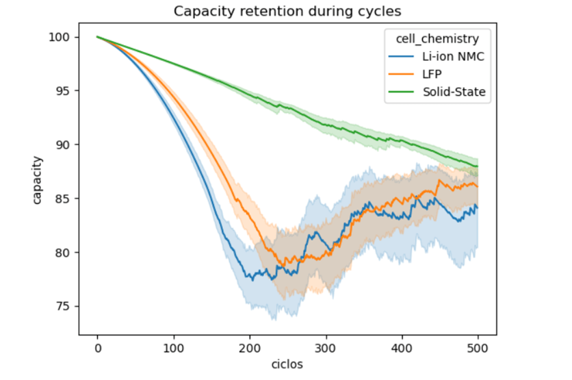
It is self-evident that the Solid state chemistry is significantly more reliable than Lithium and LFP which seem quite similar. These previous graph is quite illustrative, and one should add an extra layer of analysis; it should be done in a standardized fashion. By means of the Central Limit Theorem, one can take random samples of the global population, and obtain an bell shaped curve.

			
lithium=[]
for i in range(10000):
    								   lithium_array=np.random.choice(Li['capacity_retention_%'],size=100,replace=True)
   	 		lithium_array_mean=np.mean(lithium_array)
    			lithium.append(lithium_array_mean)
lithium=np.sort(lithium)  
lfp_norm=[]
for i in range(10000):
    lfp_array=np.random.choice(lfp['capacity_retention_%'],size=100,replace=True)
    lfp_array_mean=np.mean(lfp_array)
    lfp_norm.append(lfp_array_mean)
lfp_norm=np.sort(lfp_norm)

		

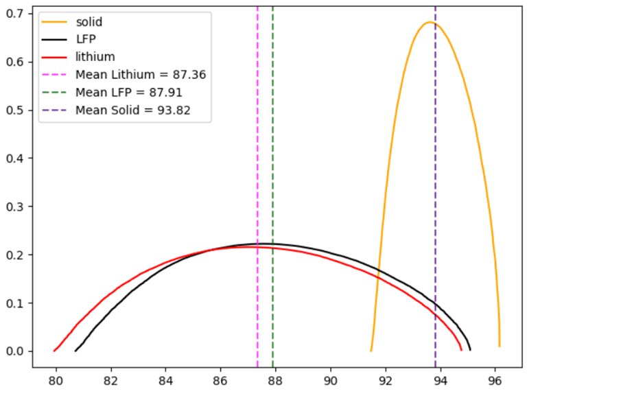
Figure 2 Standardized plots of each chemistry

Through this standard form one can get a better grasp of the differences of the three chemistries. It can be confirmed now that Solid Chemistry is absolutely more competent than the remaining two.

Mean	Standard deviation	Chemistry
93.82	0.58	Solid -State
87.32	1.83	Lithium
87.90	1.79	LFP

Table 1 Parameters for the standardized distributions of the three chemistries

What is the solid state performance vis a vis lithium?

With the assistance of the Z-score formula $Z=(X-μ)/σ$ , one may compute where does the mean solid lie in regards to the spread of the lithium data (standard deviation); solid state chemistry takes the x- value, and get that the solid state battery lies 3.52 standard deviations ahead of the lithium mean; another interpretation is to position the solid mean within the upper .02% of the lithium set. Between Lithium and LFP there is no significant difference in this performance. An additional plus for the solid is the narrowness of distribution contrasting the wideness of the spread of the other two. Thus having better process capacity. As figure 1 portrayed, there is a stark collapse in capacity in LFP or Lithium batteries, this situation merits greater depth in its causalities. For this objective, a Response Surface Methodology will be utilized.

			
SEED = 42
np.random.seed(SEED)
 
FACTORES = ['charge_rate_C', 'discharge_rate_C', 'cell_temperature_C',
            'internal_resistance_mOhm', 'irreversible_damage_index']
COVARIABLE = 'cycle'
TODOS = FACTORES + [COVARIABLE]
RESPUESTA = 'capacity_retention_%'
 
LABELS = {
    'charge_rate_C'            : 'Charge Rate (C)',
    'discharge_rate_C'         : 'Discharge Rate (C)',
    'cell_temperature_C'       : 'Temperatura (°C)',
    'internal_resistance_mOhm' : 'Resistencia Interna (mOhm)',
    'irreversible_damage_index': 'Daño Irreversible',
    'cycle'                    : 'Ciclo'
}
 
COLORES = {'Li-ion NMC': '#FF8F00', 'LFP': '#2E7D32'}
bateria_rms=bateria[(bateria['cell_chemistry']=='LFP')|(bateria['cell_chemistry']=='Li-ion NMC')]
C
# 2. FUNCIÓN RSM — reusable chemistry
# -----------------------------------------------------------------------------
def ajustar_RSM(nombre, df_q, n_max=50000, seed=SEED):
    print(f"\n{'='*65}")
    print(f"RSM — {nombre} | RESPUESTA: capacity_retention_%")
    print(f"{'='*65}")
    print(f"Registros totales : {len(df_q):,}")
    print(f"Retención media   : {df_q[RESPUESTA].mean():.2f}%")
    print(f"Retención std     : {df_q[RESPUESTA].std():.2f}%")
    print(f"Rango             : {df_q[RESPUESTA].min():.2f}% – {df_q[RESPUESTA].max():.2f}%")
 
    # Submuestreo estratificado por rango de retención
    df_q = df_q.copy()
    df_q['ret_bin'] = pd.cut(df_q[RESPUESTA],
                              bins=[0,60,70,80,85,90,95,100],
                              labels=['0-60','60-70','70-80','80-85',
                                      '85-90','90-95','95-100'])
    prop   = df_q['ret_bin'].value_counts(normalize=True)
    muestra = []
    for bin_label, proporcion in prop.items():
        n_bin = max(int(n_max * proporcion), 50)
        sub   = df_q[df_q['ret_bin'] == bin_label]
        muestra.append(sub.sample(n=min(n_bin, len(sub)), random_state=seed))
    df_m = pd.concat(muestra).sample(frac=1, random_state=seed).reset_index(drop=True)
 
    print(f"Submuestreo       : {len(df_m):,} registros (estratificado)")
 
    X = df_m[TODOS].astype(float)
    y = df_m[RESPUESTA].astype(float)
 
    X_tr, X_te, y_tr, y_te = train_test_split(X, y, test_size=0.30, random_state=seed)
 
    # Pipeline
    pipe = Pipeline([
        ('scaler', StandardScaler()),
        ('poly',   PolynomialFeatures(degree=2, include_bias=False)),
        ('model',  LinearRegression())
    ])
    pipe.fit(X_tr, y_tr)
 
    y_pred_tr = pipe.predict(X_tr)
    y_pred_te = pipe.predict(X_te)
    r2_tr  = r2_score(y_tr, y_pred_tr)
    r2_te  = r2_score(y_te, y_pred_te)
    rmse   = np.sqrt(mean_squared_error(y_te, y_pred_te))
    cv     = cross_val_score(pipe, X, y, cv=5, scoring='r2', n_jobs=-1)
 
    print(f"\n--- MÉTRICAS ---")
    print(f"R² Train          : {r2_tr:.4f}")
    print(f"R² Test           : {r2_te:.4f}")
    print(f"RMSE Test         : {rmse:.4f}%")
    print(f"CV R² (5-fold)    : {cv.mean():.4f} ± {cv.std():.4f}")
 
    # Coeficientes
    poly_step  = pipe.named_steps['poly']
    model_step = pipe.named_steps['model']
    feat_names = poly_step.get_feature_names_out(TODOS)
    coefs      = model_step.coef_
    intercepto = model_step.intercept_
 
    coef_df = pd.DataFrame({
        'termino'    : feat_names,
        'coeficiente': coefs,
        'abs_coef'   : np.abs(coefs)
    }).sort_values('abs_coef', ascending=False)
 
    # Separar efectos
    lineales      = coef_df[~coef_df['termino'].str.contains(' ') &
                             ~coef_df['termino'].str.contains('^2', regex=False)]
    cuadraticos   = coef_df[coef_df['termino'].str.contains('^2', regex=False)]
    interacciones = coef_df[coef_df['termino'].str.contains(' ') &
                             ~coef_df['termino'].str.contains('^2', regex=False)]
 
    print(f"\n--- EFECTOS LINEALES ---")
    print(f"  Intercepto: {intercepto:.4f}")
    for _, row in lineales.iterrows():
        signo = '+' if row['coeficiente'] > 0 else ''
        print(f"  {row['termino']:<40} {signo}{row['coeficiente']:.4f}")
 
    print(f"\n--- EFECTOS CUADRÁTICOS (curvatura) ---")
    for _, row in cuadraticos.iterrows():
        signo = '+' if row['coeficiente'] > 0 else ''
        print(f"  {row['termino']:<40} {signo}{row['coeficiente']:.4f}")
 
    print(f"\n--- INTERACCIONES (top 5) ---")
    for _, row in interacciones.head(5).iterrows():
        signo = '+' if row['coeficiente'] > 0 else ''
        print(f"  {row['termino']:<40} {signo}{row['coeficiente']:.4f}")
 
    # Optimización
    n_grid = 15
    grilla = {f: np.linspace(df_q[f].quantile(0.05),
                              df_q[f].quantile(0.95), n_grid) for f in FACTORES}
    grilla[COVARIABLE] = [df_q[COVARIABLE].median()]
    from itertools import product
    combos    = list(product(*[grilla[f] for f in TODOS]))
    df_grilla = pd.DataFrame(combos, columns=TODOS)
    if len(df_grilla) > 200000:
        df_grilla = df_grilla.sample(200000, random_state=seed)
    df_grilla['pred'] = pipe.predict(df_grilla[TODOS])
    opt = df_grilla.loc[df_grilla['pred'].idxmax()]
 
    print(f"\n--- CONDICIONES ÓPTIMAS (cycle fijo en mediana={df_q[COVARIABLE].median():.0f}) ---")
    for f in FACTORES:
        print(f"  {LABELS[f]:<35}: {opt[f]:.3f}")
    print(f"  Retención predicha máxima : {opt['pred']:.2f}%")
    print(f"  Retención media observada : {df_q[RESPUESTA].mean():.2f}%")
    print(f"  Ganancia sobre la media   : +{opt['pred'] - df_q[RESPUESTA].mean():.2f}%")
 
    return {
        'nombre'    : nombre,
        'pipe'      : pipe,
        'coef_df'   : coef_df,
        'lineales'  : lineales,
        'cuadraticos': cuadraticos,
        'interacciones': interacciones,
        'intercepto': intercepto,
        'r2_te'     : r2_te,
        'rmse'      : rmse,
        'cv'        : cv,
        'opt'       : opt,
        'df_q'      : df_q,
        'y_te'      : y_te,
        'y_pred_te' : y_pred_te,
        'residuales': y_te.values - y_pred_te
    }
# -----------------------------------------------------------------------------
# 3. AJUSTAR MODELOS
# -----------------------------------------------------------------------------
df_nmc = df[df['cell_chemistry'] == 'Li-ion NMC'].copy()
df_lfp = df[df['cell_chemistry'] == 'LFP'].copy()
 
res_nmc = ajustar_RSM('Li-ion NMC', df_nmc)
res_lfp = ajustar_RSM('LFP',        df_lfp)
=================================================================
RSM — Li-ion NMC | RESPUESTA: capacity_retention_%
=================================================================
Registros totales : 127,884
Retención media   : 87.36%
Retención std     : 18.40%
Rango             : 0.00% – 99.99%
Submuestreo       : 49,997 registros (estratificado)
--- MÉTRICAS ---
R² Train          : 0.9180
R² Test           : 0.9215
RMSE Test         : 4.2308%
CV R² (5-fold)    : 0.9189 ± 0.0025
In the lithium case we have that the RSM output model accounts for 92% of the variation in the response variable
--- EFECTOS LINEALES ---
  Intercepto: 88.6471
  irreversible_damage_index                -7.0603
  internal_resistance_mOhm                 -4.6517
  cycle                                    -3.1735
  charge_rate_C                            -2.4596
  discharge_rate_C                         -0.3770
  cell_temperature_C                       -0.0774
--- EFECTOS CUADRÁTICOS (curvatura) ---
  internal_resistance_mOhm^2               -2.2649
  cycle^2                                  +1.1885
  discharge_rate_C^2                       -0.1820
  irreversible_damage_index^2              +0.1305
  charge_rate_C^2                          +0.0887
  cell_temperature_C^2                     +0.0122
--- INTERACCIONES (top 5) ---
  internal_resistance_mOhm irreversible_damage_index +1.2444
  charge_rate_C irreversible_damage_index  +0.4329
  charge_rate_C cycle                      -0.3362
  irreversible_damage_index cycle          +0.3153
  discharge_rate_C cycle                   -0.2325
--- CONDICIONES ÓPTIMAS (cycle fijo en mediana=159) ---
  Charge Rate (C)                    : 0.500
  Discharge Rate (C)                 : 0.500
  Temperatura (°C)                   : 26.297
  Resistencia Interna (mOhm)         : 34.920
  Daño Irreversible                  : 0.000
  Retención predicha máxima : 98.69%
  Retención media observada : 87.36%
  Ganancia sobre la media   : +11.33%

		

All  of  the variables hold a negative relation with the % capacity. Both damage index and resistance have a negative impact on the capacity at the individual level and in coupling interactions.

=================================================================

RSM — LFP | RESPUESTA: capacity_retention_%

=================================================================

Registros totales : 159,338

Retención media   : 87.91%

Retención std     : 17.97%

Rango             : 0.00% – 99.99%

Submuestreo       : 49,996 registros (estratificado)

--- MÉTRICAS ---

R² Train          : 0.9119

R² Test           : 0.9137

RMSE Test         : 4.3846%

CV R² (5-fold)    : 0.9122 ± 0.0018

In the case of the Lfp battery, the model explains 91% of the variables

--- EFECTOS LINEALES ---

  Intercepto: 89.7591

  irreversible_damage_index                -9.1769

  internal_resistance_mOhm                 -4.5150

  cycle                                    -2.7876

  charge_rate_C                            -2.3995

  discharge_rate_C                         -0.3559

  cell_temperature_C                       -0.1349

--- EFECTOS CUADRÁTICOS (curvatura) ---

  internal_resistance_mOhm^2               -3.4782

  cycle^2                                  +1.0695

  charge_rate_C^2                          -0.4634

  irreversible_damage_index^2              -0.2764

  discharge_rate_C^2                       +0.0295

  cell_temperature_C^2                     -0.0205

--- INTERACCIONES (top 5) ---

  internal_resistance_mOhm irreversible_damage_index +3.2411

  charge_rate_C irreversible_damage_index  +0.7403

  internal_resistance_mOhm cycle           +0.5884

  discharge_rate_C internal_resistance_mOhm +0.4751

  discharge_rate_C irreversible_damage_index -0.3603

--- CONDICIONES ÓPTIMAS (cycle fijo en mediana=199) ---

  Charge Rate (C)                    : 0.500

  Discharge Rate (C)                 : 0.500

  Temperatura (°C)                   : 33.354

  Resistencia Interna (mOhm)         : 41.891

  Daño Irreversible                  : 0.000

  Retención predicha máxima : 98.39%

  Retención media observada : 87.91%

  Ganancia sobre la media   : +10.48%

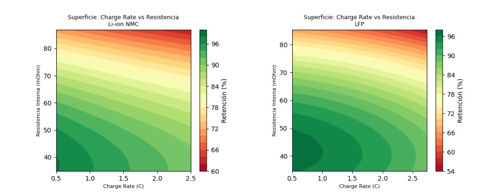
As in the lithium battery one gets that the damage index and resistance are highest ranking triggers.

Graphic Surface with optimal parameters

Figure 3 Response surface defined by charge rate and Resistance. The Lfp has little more tolerance for resistance and charge rate.

II. CTQ SAFETY/Thermal runaway

			
ciclos=bateria['cycle']
fuga=bateria['thermal_runaway_risk_score']
sns.lineplot(data=bateria, x=ciclos,y=fuga, hue='cell_chemistry')
plt.ylabel('damage')
plt.xlabel('exposure')
plt.title('thermal runaway/cycle')
plt.show()

		

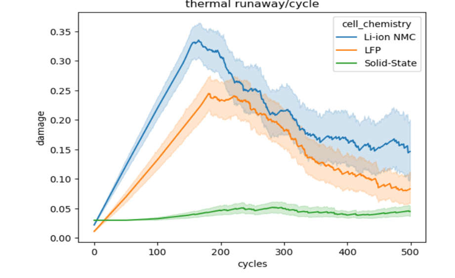
Figure 4: Thermal runaway average per cycle

A plain visual inspection plot shows once again that the solid state battery grants safer conditions. Both lithium and phosphate show signs of weariness even before reaching their half-life. For the safety concern, the analysis will focus solely in the solid state battery, because of the overwhelming security it provides along the operation. Given its safety, one should ask what are the conditions that will induce the thermal runaway. What connection does the thermal runaway hold with the other 10 variables? The most straight forward technique will be to assess the linear relationship of such response variable.

			
solid_heat_map = solid.select_dtypes(include=[np.number])
solid_na=solid_heat_map.dropna()
solid_na.drop('cumulative_high_temp_cycles', axis =1, inplace = True)
corr_solid = solid_na.corr()
diagonal_solid = np.triu(np.ones_like(corr_solid, dtype=bool))
plt.figure(figsize=(15, 13))
sns.heatmap(
    corr_solid,
    mask=diagonal_solid,
    cmap='coolwarm',
    annot=True,
    fmt=".2f",
    square=True,
    linewidths=.5,
    cbar_kws={"shrink": .8}
)
plt.title('Correlation Heatmap-solid state (Lower Triangle)')
plt.show()

		

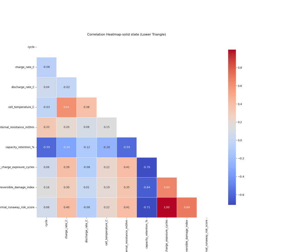
Figure 5: Heatmap of the Solid state battery

According to the last line there are two strong correlations: irreversible damage index and charge exposure cycle. A 1:1 relation would not be useful, because it will just replace the thermal runaway without adding additional value; lastly the irreversible_damage_index, as one might expect, has a strong linear linkage. The second layer of analysis will evaluate the interplay between the factors and its bearing upon the thermal runaway variable. The procedure will divide the thermal runaway failure in different categories:

(0.45-.60) moderate risk

(0.60-.70) high risk

(0.70-.80) severe risk

(0.80-0.90) critical risk

(0.90-1) catastrophic risk

One only gets a 0,76% of unsafe batteries; which are broken down in the earlier risk labels. Applying this criteria, there are just 169 batteries with critical and catastrophic labels.

			
# Clasificar por nivel de severidad
bins   = [0.45, 0.60, 0.70, 0.80, 0.90, 1.01]
labels = ['0.45-0.60 (moderado)', '0.60-0.70 (alto)',
          '0.70-0.80 (severo)',   '0.80-0.90 (crítico)',
          '0.90-1.00 (catastrófico)']
risk['severidad'] = pd.cut(risk['thermal_runaway_risk_score'],
                            bins=bins, labels=labels)
 
RESPUESTA = 'thermal_runaway_risk_score'
 
print("=" * 65)
print("PERFIL INTERNO DE FALLOS — SOLID-STATE")
print("=" * 65)
print(f"Casos analizados: {len(risk):,} (thermal_runaway >= 0.45)")
print(f"\nDistribución por severidad:")
for lab, n in risk['severidad'].value_counts().sort_index().items():
  	 pct = n / len(risk) * 100
   	 print(f"  {lab:<35}: {n:>4} ({pct:.1f}%)")

		

What drives the battery failure?

Once again, the application of the correlation coefficients will be used exclusively in those 1462 faulty cases

=================================================================

PERFIL INTERNO DE FALLOS — SOLID-STATE

=================================================================

Casos analizados: 1,463 (thermal_runaway >= 0.45)

Distribución por severidad:

0.45-0.60 (moderado) : 882 (60.3%)

0.60-0.70 (alto) : 270 (18.5%)

0.70-0.80 (severo) : 141 (9.6%)

0.80-0.90 (crítico) : 59 (4.0%)

0.90-1.00 (catastrófico) : 110 (7.5%)

			
# 5. ÁRBOL DE REGRESIÓN — reglas de severidad
# -----------------------------------------------------------------------------
print(f"\n{'='*65}")
print("ÁRBOL DE REGRESIÓN — REGLAS DE SEVERIDAD")
print(f"{'='*65}")
 
cart_reg = DecisionTreeRegressor(max_depth=3, random_state=SEED,
                                  min_samples_leaf=20)
cart_reg.fit(X, y)
 
print(export_text(cart_reg, feature_names=[LABELS[f] for f in FACTORES]))
 
imp = pd.Series(cart_reg.feature_importances_,
                index=[LABELS[f] for f in FACTORES]).sort_values(ascending=False)
print("IMPORTANCIA DE VARIABLES (árbol de regresión):")
for var, val in imp.items():
    if val > 0:
        barra = '█' * int(val * 40)
        print(f"  {var:<35}: {val:.4f}  {barra}")
=================================================================
ÁRBOL DE REGRESIÓN — REGLAS DE SEVERIDAD
=================================================================
|--- Resistencia Interna (mOhm) <= 106.81
|   |--- Charge Rate (C) <= 3.01
|   |   |--- Charge Rate (C) <= 2.76
|   |   |   |--- value: [0.46]
|   |   |--- Charge Rate (C) >  2.76
|   |   |   |--- value: [0.47]
|   |--- Charge Rate (C) >  3.01
|   |   |--- Resistencia Interna (mOhm) <= 73.04
|   |   |   |--- value: [0.52]
|   |   |--- Resistencia Interna (mOhm) >  73.04
|   |   |   |--- value: [0.63]
|--- Resistencia Interna (mOhm) >  106.81
|   |--- Resistencia Interna (mOhm) <= 130.04
|   |   |--- Charge Rate (C) <= 3.36
|   |   |   |--- value: [0.66]
|   |   |--- Charge Rate (C) >  3.36
|   |   |   |--- value: [0.83]
|   |--- Resistencia Interna (mOhm) >  130.04
|   |   |--- Resistencia Interna (mOhm) <= 141.68
|   |   |   |--- value: [0.94]
|   |   |--- Resistencia Interna (mOhm) >  141.68
|   |   |   |--- value: [1.00]
IMPORTANCIA DE VARIABLES (árbol de regresión):
  Resistencia Interna (mOhm)         : 0.8742  ██████████████████████████████████
  Charge Rate (C)                    : 0.1258  █████

		

As one might appreciate from the previous decision tree, when the resistance increases above 130 combustion is basically a fait accompli.

One now grasps which variables induce the greatest thermal risk in the battery; for the sake of achieving greater formality, an FMEA (Failure mode and effects analysis) will be executed basing it on the 5 failure criteria; the probability will be calculated on the incidence within the 1463 population.

FMEA occurrence

Mode	Cases	%	Occurrence	Description
Moderate	882	60.3%	8	Very frequent
High	270	18.5%	6	frequent
Severe	141	9.6%	5	moderate
Critical	59	4.0%	3	unfrequent
Catastrophic	110	7.5%	4	rare

Table 3 occurrence

Detection values will be assigned based on the measurability of the key variables identified in the regression tree. Internal resistance and charge rates are continuously monitored parameters in modern Battery Management Systems, granting hight detectability at lower security levels. As severity escalates the window for detection will narrow.

Failure mode	Severity	Occurrence	Detection	npr
Catastrophic	10	4	6	240
Severe	7	5	4	140
Moderate	5	8	2	80
High	6	6	3	108
Critical	8	3	5	120

Table 4 FMEA

Given the figure 5 output and the decision tree, one gets the following criteria for the 5 classifications:

-Moderate , RPN=80

Key variable: charge rate

Threshold: charge rate > 3.01

Action: Establish a charge rate limit of 3.01

-High, RPN 108

Key variable: internal resistance and charge rate

Threshold: Resistance above 73

Action: raise cautionary flag at 73 mohms

-Severe, RPN 140

Key variable : internal resistance

Threshold: Resistance above 107

Action: Reduce charge

-Critical, RPN 120

Key variable: charge rate + internal resistance

Secondary variable: irreversible damage index

Threshold: Resistance > 107 and charge rate >3.36

Action: immediate charge suspension

-Catastrophic, RPN 240

Key variable: Internal resistance

Threshold: internal resistance > 130

Action: Suspend operation replace unit

A swift recapitulation of the previous work: departing from market requirements, one find its respective critical to quality engineering counterpart. The first step is compare the batteries according to its three different chemistries. The following outcomes are achieved:

Through the statistical Response Surface Methodology technique one gets which variables can be manipulated in order to monitor the performance. The model has more than 90% precision.
From a very brief visualization is quite clear that the solid state battery is far more competent in terms of its capacity retention. The distance between standardized means statistically proves this. When it comes to safety, the solid state battery has greater lifespan and less risks
Both CTQ´s can be monitored through the assessment of the same variables which can simplify the assurance job (resistance, charge rate and irreversible damage index) besides the obvious time frame or cycle.

Quality Control does not end at the shipping dock inside the manufacturing facility; it involves post-sales service and proper usage counselling for the user; always aiming at maximizing lifespan and minimizing costs. Through Quality function Design the consumer can grant itself with valuable cautionary points that will assist him or her in achieving the purported goals for which, in this case, the battery was acquired.

Quality Function Design of electric batteries through Data Analysis

What People want in electric car batteries?(source: More than 50% of drivers expect to own an electric car by 2034)

What defines such Quality?

What is the solid state performance vis a vis lithium?

Graphic Surface with optimal parameters

What drives the battery failure?

Comparte esto:

Deja un comentario Cancelar la respuesta