The defraying of logistical expenditures can be a challenge, specially, in face of short term cash obligations. Companies can resort to factoring mechanisms that will grant them credit for their monthly import operations; for such service providers keeping historical records is of paramount relevance.Ergo, one can manage risk involved in money lending. The dataset containing the credit customer data spans over a 4 month period, the amount of money lent varies from customer to customer.

The purpose of this entry is to apply Markov chains knowledge into the debtors behaviour . All debtors are divided into four groups: AAA, when the debt is liquidated within 30 days after its emission; AA, when the debt is liquidated within 60 days; B, when the total amount is paid within 90 days; Bad debt, subdivided itself into two: C, when the accounts are transfered, throughout a 30 day period, to a collection agency which will add a surcharge to each unit of debt retrieved of $ 800,00; D, when the debt is not paid with the agency assistance, and more aggressive action will need to take place. The raw dataset will contain information from the debtors for the first trimester of 2021. Each group or state will be characterised for its fluidity with the notorious exception of Bad debt (C and D) which are absorbent states; customers can move through the remaining states depending on the punctuality of payments along the different emissions. Due to the categorical and binary nature of the debt status (paid or unpaid), one ought to employ zeroes and ones to label the four milestone-payment dates along the data. Once the customer-debtor has paid his dues, his credit line is renewed by the following month. One, thus, must find four different cash streams with their respective four month margin.

Applying the python pandas library, one can start making sense of the untidy dataset in form of an Microsoft Excel file. One shall begin with getting the number of entitities in the dataset.

 pandas as pd
import numpy as np
pd.read_csv(r'C:\Users\Alonso\Documents\given credit 2021.csv')
tot_debtot_debtorsors=credit_dataset["num"].nunique()
6409

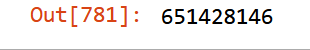
Another step for outlining the data will be to calculate the total capital at disposal.

credit_dataset["credit_amount"].sum()

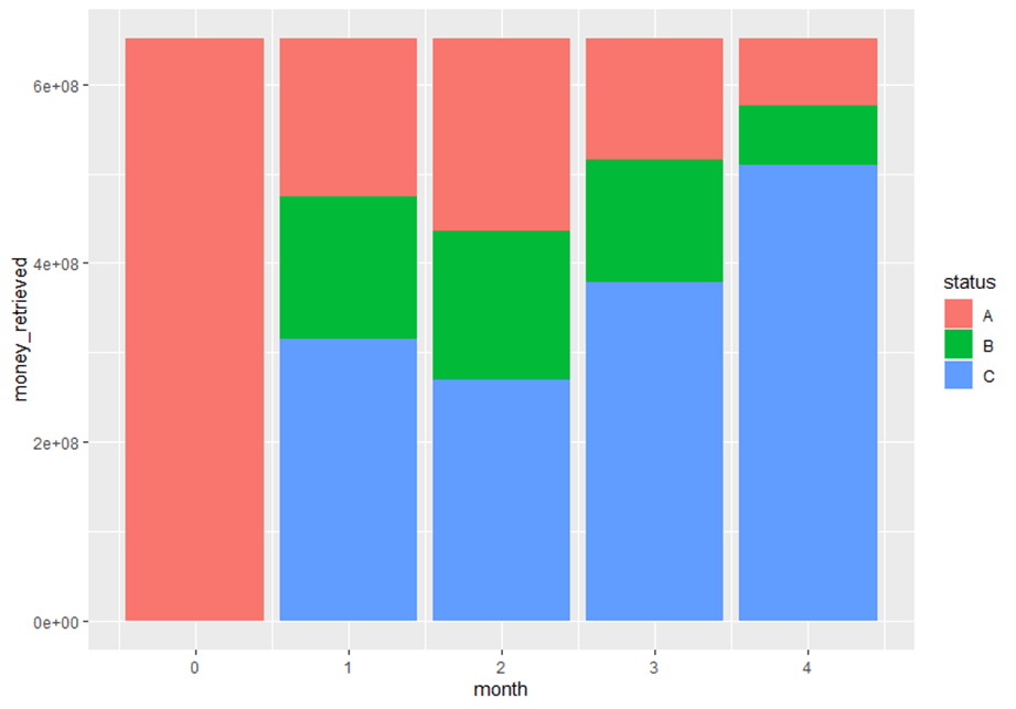
As previously mencioned, the determination of payment punctuality by every date milestone is labeled with «0» and «1». So, by adding each column one can get the distribution of customers in different dates.

AAA_debtors=credit_dataset[«first_date»].sum()

credit_dataset_df=pd.DataFrame(credit_dataset)

AA_debtors=credit_dataset_df["second_date"].sum()
AA_debtors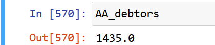

B_debtors=credit_dataset[«third_date»].sum()
B_debtors

Bad Debt estimation

Because of the dual nature of Bad debt, Pivot tables will be used to separate the two types, those who pay once the Collection agency makes contact,»C», and the ones who even after that fall into arrears with «0» in the fourth date.

credit_dataset.pivot_table(values="credit_utilized",columns="fourth_date",aggfunc="count")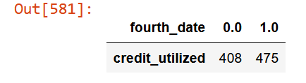

A Markov Chain is a type of stochastic process in which a variable varies across time into a finite set of states; this variation´s core tenet is that future states depend solely on the current state. The input element for the markov chain is the Transition matrix; such array will provide us with the probability to which customers can move from one credit status to another; this movements will be sourced from payment punctuality during the following 4 months.

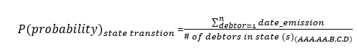
Using pivot tables one can estimate the punctuality ratio based upon previously calculated states using the following expression arranged in a matrix fashion:

Using the following code:

transition_matrix=np.matrix([[credit_dataset["first_date_second_emission"].sum()/AAA_debtors,credit_dataset["second_date_second_emission"].sum()/AAA_debtors,credit_dataset["third_date_second_emission"].sum()/AAA_debtors,credit_dataset["fourth_date_second_emission"].sum()/AAA_debtors,credit_dataset[credit_dataset["fourth_date_second_emission"]==0]["num"].count()/AAA_debtors],[credit_dataset["first_date_third_emission"].sum()/AA_debtors,credit_dataset["second_date_third_emission"].sum()/AA_debtors,credit_dataset["third_date_third_emission"].sum()/AA_debtors,credit_dataset["fourth_date_third_emission"].sum()/AA_debtors,credit_dataset[credit_dataset["fourth_date_third_emission"]==0]["num"].count()/AA_debtors],[credit_dataset["first_date_fourth_emission"].sum()/B_debtors,credit_dataset["second_date_fourth_emission"].sum()/B_debtors,credit_dataset["third_date_fourth_emission"].sum()/B_debtors,credit_dataset["fourth_date_fourth_emission"].sum()/B_debtors,credit_dataset[credit_dataset["fourth_date_fourth_emission"]==0]["num"].count()/B_debtors],[0,0,0,1,0],[0,0,0,0,1]])

With the following output:

Debt status	AAA	AA	B	C	D
AAA	0.64	0.21	0.08	0.04	0.02
AA	0.47	0.26	0.15	0.05	0.06
B	0.48	0.33	0.08	0.05	0.04
C	0	0	0	1	0
D	0	0	0	0	1

Relevant Questions

With the prior accoutrements one can begin to make predictions and draw relevant conclusions for the decision takers.

1.What is the probability that an excellent debtor will fall into bad debt after one trimester? By a simple look at the transition matrix, one sees that around 6% of them will fall into arrears.

2.What is the probability that a debtor with initial AA will end up in B status at the end of the year?

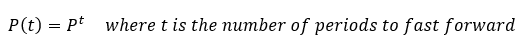
According to the succint corollary of the Kolmogorov-Chapman equations, one can impel forward any transition probabilities to future periods by just powering the transition matrix to that required period.

transition_matrix**3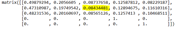

A fraction over 8% will fall into arrears within 60 and 90 days.

3. What is the estimated total cost of bad debt recollection at the end of
the year considering the 800,00 fare?

All needed to do in this point, is to add all of the fourth dates within
different emissions, which will amount to a total of $ 1.060,000

As a concluding note, one ought to make sense of that last figure in tandem with the cash availability in terms of the amount repaid, amount falling into arrears, and the amount in stock.